Class Lab 4

Review

In our dataset for this activity (lab4.dta), which again comes from the ATUS and includes time spent on a variety of activities, we have a set of indicators for race categories and income categories. For our example today, we will be working with the income variable. You will find that for some things, like graphs and two-way tables in tabulate, having categorical variables is valuable, while for other things, like creating a table for reporting outside of Stata, indicator variables are more useful.

We will begin with our usual preamble in our code:

cd "E:\rpad316\"
log using "logs\lab4.log", replace
use "data\lab4.dta"

Let’s create a categorical version household income using the indicator variables in the dataset.

As always, be sure to label both the variable and its values so you do not forget what the variable is later.

gen income = .
replace income = 1 if loinc == 1
replace income = 2 if lowmidinc == 1
replace income = 3 if himidinc == 1
replace income = 4 if inc150p == 1

label var income "HH income"
label define inccat 1 "<$20K" 2 "$20K to 60K" 3 "$60K to 150K" 4 ">$150K"
label val income inccat

Let’s practice creating a table that captures the average time spent on taking care of others, working, and socializing by income bracket using the income variable we created above. We will begin by creating variables that only includes people who spent at least some time on each activity.

gen care2 = care_tot if care_tot > 0
gen wrktime2 = wrktime if wrktime > 0
gen socialize2 = socialize_tot if socialize_tot > 0

label var wrktime2 "Time working"
label var care2 "Time caring for others"
label var socialize2 "Time socializing"

Now, let’s plug those variables into the same code we used before, in Class Lab 3, to make our conditional means table using binary indicators. For this table, we will examine time spent on these activities, in minutes, across the different income categories using the categorical variable we created.

estpost sum wrktime2 care2 socialize2 if income == 1
eststo lowinctime
estpost sum wrktime2 care2 socialize2 if income == 2
eststo lowmidinc
estpost sum wrktime2 care2 socialize2 if income == 3
eststo himidinc
estpost sum wrktime2 care2 socialize2 if income == 4
eststo highinc
estpost sum wrktime2 care2 socialize2
eststo totals
esttab lowinctime lowmidinc himidinc highinc totals using "output\example1_lab4.csv", cell(mean(fmt(2)) sd(par)) replace label unstack csv mtitles("Low income" "Lower-middle income" "Upper-middle income" "High income" "Total")

As always, replace the example1_lab4 part above with the title of the file that makes the most sense for you. The mtitles() part of the code labels the columns of the table, in order. The code should produce a table that looks like this:

What a nice table! The table shows that, on an average day, someone in the U.S. works 435.33 minutes or about 7 hours and 15 minutes. Meanwhile, the average American, on an average day during which they care for someone, spends about 115 minutes caring for the person or about 1 hour and 55 minutes. Generally, it looks like the lower-middle class spends the most time working, on average, while high income individuals spend the least time working. Similarly, both high- and low-income individuals spend about the same amount of time caring for someone else, on average.

Z-Scores

Now, as we covered, sometimes we are interested in difference between categories relative to the distribution of all values of x. We can see this by calculating z-scores for each observation, which tells us where that observation lies relative to the whole population. To compute the z-score, we just need the mean and standard deviation of the sample and we can compute a z-score for each observation.

In Stata, we can do this by creating a variable that contains the mean of our variables for the full sample and another that contains the standard deviation of the full sample. To do this, we will use egen, a special version of the generate command that can create new variables that are derived from a mathematical function of other variables. We will be using the simplest application of egen for calculating z-scores. I will use care time as the example to walk through the steps. First, create a variable equal to the sample mean of time spent caring for others:

egen mean_care = mean(care2)

This will create a variable that is equal to the mean and apply that value to every observation in your dataset. We will use egen again to do the same thing for estimating the standard deviation.

egen sd_care = sd(care2)

Now, we can use all of these components and create a variable that applies the z-score formula to each observation of x (in this case care2) in the sample. Recall that the formula for the z-score is:

\[Z = \dfrac{(X - \overline{X})}{S_x}\]

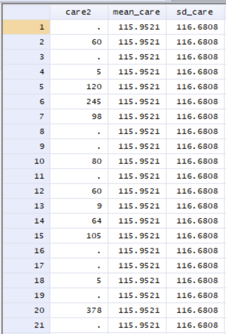
In Stata, the variables we just created look like this:

Notice that the variables we created before, mean_care and sd_care, have the same value for each observation in the dataset, and the value is equal to the sample mean of care time and the sample standard deviation of care time. We can now use each observation’s X, mean, and standard deviation to create a variable that contains the z-score of time spent caring for someone else:

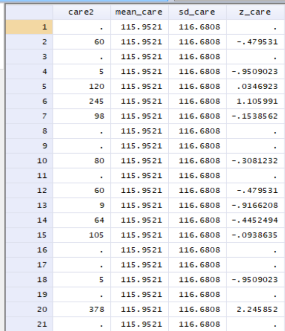
gen z_care = ((care2 - mean_care)/sd_care)

The code creates a variable that looks like this for the same set of observations:

Now, z_care contains each observation’s z-score. As a result, when we take the sample mean of z_care, it will have a mean of zero with a standard deviation of 1, reflecting the fact that it is a standardized variable expressed in terms of deviations from the mean. Let’s follow the same process for each of the other time variables we have to standardize them and create a table of their means and standard deviations to demonstrate this.

egen mean_wrktime = mean(wrktime2)
egen sd_wrktime = sd(wrktime2)
gen z_wrktime = ((wrktime2 - mean_wrktime)/sd_wrktime)


egen mean_social = mean(socialize2)
egen sd_social = sd(socialize2)
gen z_social = ((socialize2 - mean_social)/sd_social)

label var z_wrktime "Standardized work time"
label var z_care "Standardized care time"
label var z_social "Standardized social time"

Now, let’s re-create our previous table, using z-scores instead of minutes in each activity.

estpost sum z_wrktime z_care z_social if income == 1
eststo lowinctime
estpost sum z_wrktime z_care z_social if income == 2
eststo lowmidinc
estpost sum z_wrktime z_care z_social if income == 3
eststo himidinc
estpost sum z_wrktime z_care z_social if income == 4
eststo highinc
estpost sum z_wrktime z_care z_social
eststo totals
esttab lowinctime lowmidinc himidinc highinc totals using "output\example2", cell(mean(fmt(2)) sd(par)) replace label csv mtitles("Low income" "Lower-middle income" "Upper-middle income" "High income" "Total")

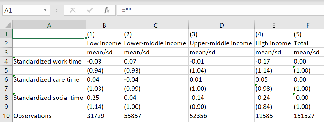
Which will make a table that looks like:

In column 5, we see that all three variables have a mean of approximately 0 and standard deviation of 1, as expected. As a result, we can more directly compare the size of the gap between income categories across all activities. We can see that, on average, high income individuals’ work time is 0.17 of a standard deviation below the average American. Meanwhile, high income individuals’ care-taking time is about 0.05 of a standard deviation above the average American. The gap between high and low income individuals is highest in socializing time, with a gap of about 0.49 of a standard deviation.

Z Scores and Z Table in Stata

Of course, as we covered in lecture 5, we can also use Z tables to take advantage of the standard properties of a normal distribution and look up population proportions at various Z scores. In Stata, pulling up a ztable is simple - simply enter ztable, c in the command window and Stata will present a Z-table for you to use:

. ztable, c

      Cumulative Area of the Standard Normal Distribution
       .00    .01    .02    .03    .04   |  .05    .06    .07    .08    .09
-3.50 0.0002 0.0002 0.0002 0.0002 0.0002 | 0.0002 0.0002 0.0002 0.0002 0.0002
-3.40 0.0003 0.0003 0.0003 0.0003 0.0003 | 0.0003 0.0003 0.0003 0.0003 0.0002
-3.30 0.0005 0.0005 0.0005 0.0004 0.0004 | 0.0004 0.0004 0.0004 0.0004 0.0003
-3.20 0.0007 0.0007 0.0006 0.0006 0.0006 | 0.0006 0.0006 0.0005 0.0005 0.0005
-3.10 0.0010 0.0009 0.0009 0.0009 0.0008 | 0.0008 0.0008 0.0008 0.0007 0.0007
-3.00 0.0013 0.0013 0.0013 0.0012 0.0012 | 0.0011 0.0011 0.0011 0.0010 0.0010
-2.90 0.0019 0.0018 0.0018 0.0017 0.0016 | 0.0016 0.0015 0.0015 0.0014 0.0014
-2.80 0.0026 0.0025 0.0024 0.0023 0.0023 | 0.0022 0.0021 0.0021 0.0020 0.0019
-2.70 0.0035 0.0034 0.0033 0.0032 0.0031 | 0.0030 0.0029 0.0028 0.0027 0.0026
-2.60 0.0047 0.0045 0.0044 0.0043 0.0041 | 0.0040 0.0039 0.0038 0.0037 0.0036
-2.50 0.0062 0.0060 0.0059 0.0057 0.0055 | 0.0054 0.0052 0.0051 0.0049 0.0048
-2.40 0.0082 0.0080 0.0078 0.0075 0.0073 | 0.0071 0.0069 0.0068 0.0066 0.0064
-2.30 0.0107 0.0104 0.0102 0.0099 0.0096 | 0.0094 0.0091 0.0089 0.0087 0.0084
-2.20 0.0139 0.0136 0.0132 0.0129 0.0125 | 0.0122 0.0119 0.0116 0.0113 0.0110
-2.10 0.0179 0.0174 0.0170 0.0166 0.0162 | 0.0158 0.0154 0.0150 0.0146 0.0143
-2.00 0.0228 0.0222 0.0217 0.0212 0.0207 | 0.0202 0.0197 0.0192 0.0188 0.0183
-1.90 0.0287 0.0281 0.0274 0.0268 0.0262 | 0.0256 0.0250 0.0244 0.0239 0.0233
-1.80 0.0359 0.0351 0.0344 0.0336 0.0329 | 0.0322 0.0314 0.0307 0.0301 0.0294
-1.70 0.0446 0.0436 0.0427 0.0418 0.0409 | 0.0401 0.0392 0.0384 0.0375 0.0367
-1.60 0.0548 0.0537 0.0526 0.0516 0.0505 | 0.0495 0.0485 0.0475 0.0465 0.0455
-1.50 0.0668 0.0655 0.0643 0.0630 0.0618 | 0.0606 0.0594 0.0582 0.0571 0.0559
-1.40 0.0808 0.0793 0.0778 0.0764 0.0749 | 0.0735 0.0721 0.0708 0.0694 0.0681
-1.30 0.0968 0.0951 0.0934 0.0918 0.0901 | 0.0885 0.0869 0.0853 0.0838 0.0823
-1.20 0.1151 0.1131 0.1112 0.1093 0.1075 | 0.1056 0.1038 0.1020 0.1003 0.0985
-1.10 0.1357 0.1335 0.1314 0.1292 0.1271 | 0.1251 0.1230 0.1210 0.1190 0.1170
-1.00 0.1587 0.1562 0.1539 0.1515 0.1492 | 0.1469 0.1446 0.1423 0.1401 0.1379
-0.90 0.1841 0.1814 0.1788 0.1762 0.1736 | 0.1711 0.1685 0.1660 0.1635 0.1611
-0.80 0.2119 0.2090 0.2061 0.2033 0.2005 | 0.1977 0.1949 0.1922 0.1894 0.1867
-0.70 0.2420 0.2389 0.2358 0.2327 0.2296 | 0.2266 0.2236 0.2206 0.2177 0.2148
-0.60 0.2743 0.2709 0.2676 0.2643 0.2611 | 0.2578 0.2546 0.2514 0.2483 0.2451
-0.50 0.3085 0.3050 0.3015 0.2981 0.2946 | 0.2912 0.2877 0.2843 0.2810 0.2776
-0.40 0.3446 0.3409 0.3372 0.3336 0.3300 | 0.3264 0.3228 0.3192 0.3156 0.3121
-0.30 0.3821 0.3783 0.3745 0.3707 0.3669 | 0.3632 0.3594 0.3557 0.3520 0.3483
-0.20 0.4207 0.4168 0.4129 0.4090 0.4052 | 0.4013 0.3974 0.3936 0.3897 0.3859
-0.10 0.4602 0.4562 0.4522 0.4483 0.4443 | 0.4404 0.4364 0.4325 0.4286 0.4247
 0.00 0.5000 0.5040 0.5080 0.5120 0.5160 | 0.5199 0.5239 0.5279 0.5319 0.5359
 0.10 0.5398 0.5438 0.5478 0.5517 0.5557 | 0.5596 0.5636 0.5675 0.5714 0.5753
 0.20 0.5793 0.5832 0.5871 0.5910 0.5948 | 0.5987 0.6026 0.6064 0.6103 0.6141
 0.30 0.6179 0.6217 0.6255 0.6293 0.6331 | 0.6368 0.6406 0.6443 0.6480 0.6517
 0.40 0.6554 0.6591 0.6628 0.6664 0.6700 | 0.6736 0.6772 0.6808 0.6844 0.6879
 0.50 0.6915 0.6950 0.6985 0.7019 0.7054 | 0.7088 0.7123 0.7157 0.7190 0.7224
 0.60 0.7257 0.7291 0.7324 0.7357 0.7389 | 0.7422 0.7454 0.7486 0.7517 0.7549
 0.70 0.7580 0.7611 0.7642 0.7673 0.7704 | 0.7734 0.7764 0.7794 0.7823 0.7852
 0.80 0.7881 0.7910 0.7939 0.7967 0.7995 | 0.8023 0.8051 0.8078 0.8106 0.8133
 0.90 0.8159 0.8186 0.8212 0.8238 0.8264 | 0.8289 0.8315 0.8340 0.8365 0.8389
 1.00 0.8413 0.8438 0.8461 0.8485 0.8508 | 0.8531 0.8554 0.8577 0.8599 0.8621
 1.10 0.8643 0.8665 0.8686 0.8708 0.8729 | 0.8749 0.8770 0.8790 0.8810 0.8830
 1.20 0.8849 0.8869 0.8888 0.8907 0.8925 | 0.8944 0.8962 0.8980 0.8997 0.9015
 1.30 0.9032 0.9049 0.9066 0.9082 0.9099 | 0.9115 0.9131 0.9147 0.9162 0.9177
 1.40 0.9192 0.9207 0.9222 0.9236 0.9251 | 0.9265 0.9279 0.9292 0.9306 0.9319
 1.50 0.9332 0.9345 0.9357 0.9370 0.9382 | 0.9394 0.9406 0.9418 0.9429 0.9441
 1.60 0.9452 0.9463 0.9474 0.9484 0.9495 | 0.9505 0.9515 0.9525 0.9535 0.9545
 1.70 0.9554 0.9564 0.9573 0.9582 0.9591 | 0.9599 0.9608 0.9616 0.9625 0.9633
 1.80 0.9641 0.9649 0.9656 0.9664 0.9671 | 0.9678 0.9686 0.9693 0.9699 0.9706
 1.90 0.9713 0.9719 0.9726 0.9732 0.9738 | 0.9744 0.9750 0.9756 0.9761 0.9767
 2.00 0.9772 0.9778 0.9783 0.9788 0.9793 | 0.9798 0.9803 0.9808 0.9812 0.9817
 2.10 0.9821 0.9826 0.9830 0.9834 0.9838 | 0.9842 0.9846 0.9850 0.9854 0.9857
 2.20 0.9861 0.9864 0.9868 0.9871 0.9875 | 0.9878 0.9881 0.9884 0.9887 0.9890
 2.30 0.9893 0.9896 0.9898 0.9901 0.9904 | 0.9906 0.9909 0.9911 0.9913 0.9916
 2.40 0.9918 0.9920 0.9922 0.9925 0.9927 | 0.9929 0.9931 0.9932 0.9934 0.9936
 2.50 0.9938 0.9940 0.9941 0.9943 0.9945 | 0.9946 0.9948 0.9949 0.9951 0.9952
 2.60 0.9953 0.9955 0.9956 0.9957 0.9959 | 0.9960 0.9961 0.9962 0.9963 0.9964
 2.70 0.9965 0.9966 0.9967 0.9968 0.9969 | 0.9970 0.9971 0.9972 0.9973 0.9974
 2.80 0.9974 0.9975 0.9976 0.9977 0.9977 | 0.9978 0.9979 0.9979 0.9980 0.9981
 2.90 0.9981 0.9982 0.9982 0.9983 0.9984 | 0.9984 0.9985 0.9985 0.9986 0.9986
 3.00 0.9987 0.9987 0.9987 0.9988 0.9988 | 0.9989 0.9989 0.9989 0.9990 0.9990
 3.10 0.9990 0.9991 0.9991 0.9991 0.9992 | 0.9992 0.9992 0.9992 0.9993 0.9993
 3.20 0.9993 0.9993 0.9994 0.9994 0.9994 | 0.9994 0.9994 0.9995 0.9995 0.9995
 3.30 0.9995 0.9995 0.9995 0.9996 0.9996 | 0.9996 0.9996 0.9996 0.9996 0.9997
 3.40 0.9997 0.9997 0.9997 0.9997 0.9997 | 0.9997 0.9997 0.9997 0.9997 0.9998
 3.50 0.9998 0.9998 0.9998 0.9998 0.9998 | 0.9998 0.9998 0.9998 0.9998 0.9998

What if we don’t have data and want to calculate the z-score from a mean, standard deviation, and X value? In Stata, there is a user written package, zcalc, that allows us to calculate a z-score in Stata if we ever need to use it for anything. We will have to run a quick search in Stata for it though:

findit zcalc

We should get a results page that looks like this:

If we click on the zcalc link, it will take us to the package installation page. Here, we simply click “click here to install” and Stata will install zcalc for us.

Now, let’s use it to find a z-score associate with 700 minutes working using the mean and standard deviation we estimated in table 1 of our exercise. To do it, we simply list the X-value, mean, and standard deviation in order - zcalc 700 435.33 201.09 - which will produce an output like this:

. zcalc 700 435.33 201.09

z-score for sample observations

      (X - m)       (700 - 435.33)
 z = ---------  =  ------------------  =  1.32
         s              201.09

As we can see, someone who works 700 minutes in a typical day, or a little over 11 and a half hours, is 1.32 standard deviations above the average Americans’ work time. Looking at the Z-table above, someone working 700 minutes in a given day is spending more time working that 90.49% of Americans.