
Exercise 4
Summarizing variables and making tables
One of the key starting points of analyzing data for research is examining the central tendancy and distribution (or spread) of the variables of immediate interest to the study. In this lab, we will walk through how to think about summarizing a variable and a relationship between two variables with a few simple graphs, summarizing several variables in a sample, and then creating tables we can use in our research reports. We will do this using data from the American Time Use Survey once again and we’ll explore two broad outcomes: time spent alone and the effect of a young children on time use patterns.
Installing Packages
Before we begin, however, we need to install a few user-created packages that will let us look at our data in a clear way and then create nice, clean tables after we run some analysis.
First, we will install fre which is short for “frequency.” This command allows us to see tabulations of the values and labels of categorical variables in one place with a single command - a very useful and convenient need when we are first assessing variables in our data. To install it, simply run:
ssc install fre, replace
The ssc install command searches the STATA package repository, finds fre and installs it for use on your computer. You only need to do this once and you are good to go.
Next, we need to install the estout package, which includes a suite of commands that allow us to store estimates in STATA’s temporary memory and then output them into formatted tables for use in Word, Excel, or a number of other formats. The process is the same:
ssc install estout, replace
Now we have the tools we need to get going on looking at variables and making tables!
Some Simple Graphs
Aging and Loneliness
Let’s start with looking at the relationship between time spent alone and age. We might expect that as people age, they spend more time alone and given the effect of excess loneliness on mental health, this might be something we would be concerned about and could try to counteract with programs, volunteers, and other means. Both of these are continuous variables, so plotting the relationship between them using a scatter plot is sensible and appropiate. We will add some wrinkles to this as we go, but let’s start with the basics - simple scatter plot.
scatter trtalone teage
graph export "output\scatter1.png", replace
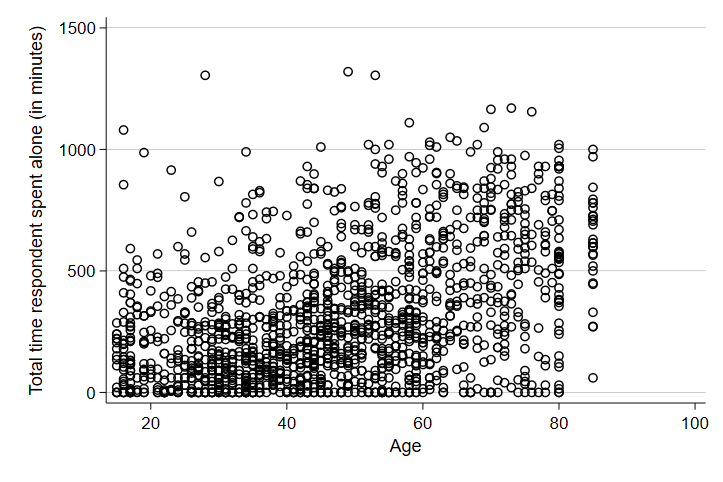
Note that the first line of the code generates the scatter plot and the second line tells STATA to save the graph as an image in my output folder. PNG files are useful and flexible - you can drag and drop them into work, text them as pictures, or add them to websites.
As we might have predicted, there seems to be a slightly positive, weak relationship between age and the minutes someone spends alone on a typical day. Let’s see if it varies by gender.
scatter trtalone teage, by(tesex)
graph export "output\scatter2.png", replace
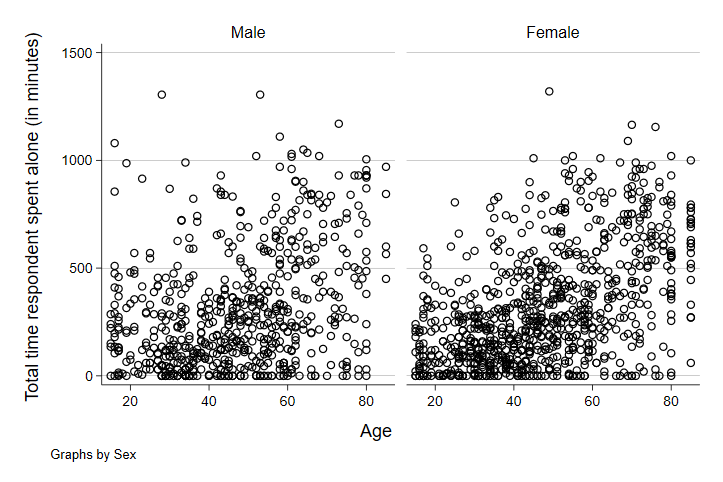
Hm. It seems like it might - there seems to be a slightly stronger relationship between the two in the female side of the graph, but it’s too hard to tell from the plots alone. Let’s add the best-fit line to each of these and see how that looks. The best-fit line will show us the slope of the relationship between age and minutes spent alone on a typical day. It will also give us a better visual cue - as steeper line will give us some indication that the relationship is stronger.
scatter trtalone teage, by(tesex) || lfit trtalone teage, by(tesex) lcolor(red)
graph export "output\scatter3.png", replace
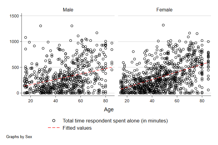
Note that we added the two vertical lines (||). In STATA graphs, this can be used to overlay graphs. Everything after this part of the code is the instructions on what variables should define the line and how to mark the line to make it visible (in this case, changing the color to red). As we can see, there does seem to be a stronger relationship between time alone and age among women than men. Note though that there are more observations among women at the older end of the age distribution - likely driven in part by women living longer, on average, than men. At least some of the stronger relationship here is likely related to this difference.
Beyond gender, we might also consider whether income matters for time spent alone. Higher income corresponds to wide variety of other benefits - from mental and physical health to family stability and life satisfaction. Before we try to graph this, let’s take a look at the categorical variable income_cat in our dataset with our handy new command fre:
fre income_cat

income_cat -- HH income
----------------------------------------------------------------------
                         |      Freq.    Percent      Valid       Cum.
-------------------------+--------------------------------------------
Valid   1 < $20K         |        371      24.73      24.73      24.73
        2 $20K to $40K   |        345      23.00      23.00      47.73
        3 $40K to 60K    |        240      16.00      16.00      63.73
        4 $60K to 75K    |        137       9.13       9.13      72.87
        5 $75K to $100K  |        176      11.73      11.73      84.60
        6 $100K to $150K |        121       8.07       8.07      92.67
        7 > $150K        |        110       7.33       7.33     100.00
        Total            |       1500     100.00     100.00
----------------------------------------------------------------------
Here, we can see we have seven categories of income. We don’t want to look at 7 different scatterplots - that’s a lot to take in at once - so let’s make things easy on ourselves and create a binary variable that identifies only the richest and poorest households in our data. For this, instead of using gen and replace like we did in our previous excercise, we are going to learn a new command called recode. Recode is a useful command for collapsing a categorical variable with many categories into a smaller number of categories.
recode income_cat (1 = 1 "Low-income") (7 = 2 "High-income") (2/6 = .), gen(hilowinc)
label var hilowinc "High- and Low-income"
In the code above, each statement in parentheses is used for a new category. In the first, we tell STATA to use the first category in the original variable and to set it to be the first value in our new variable with a new label of “Low-income.” The second, we take the 7th category of the original variable, the highest income bracket, and make it the second category in our new variable with a new label. Finally, demonstrating the flexibility of recode, we set all values from 2 to 6 in the original variable (the / tells STATA that this should be all numeric values between these two values) to be missing values in the new vairable. Finally, in our option section (the part of the code past the comma), we tell STATA to create a new variable called hilowinc with those new categories. The second line of code labels our new variable for a more intuitive reminder of what this variable is telling us.
Now we’re ready to look at the relationship between age and time spent alone on a typical day separately by high and low income.
scatter trtalone teage, by(hilowinc) || lfit trtalone teage, by(hilowinc) lcolor(red)
graph export "output\scatter4.png", replace
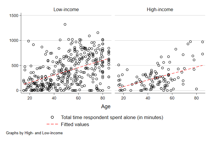
Here, we can see that unlike with gender, the strength of the relationship between time alone and age is pretty similar across low- and high-income people. The slope is about the same - the line is just higher among low-income people, which tells us that low-income people spend more time alone in a typical day on average at each age.
Children and Time Use Patterns
In addition to simple aging, having a child can alter how we spend our time dramatically. Importantly, looking at households that have young children and those that don’t gives us a chance to look at some graphs that show the relationship between a continuous variable (time) and a categorical variable (whether someone has a child less than two years old or not). Let’s start by looking at the distribution of a few time use variables. We’ll start with work time.
hist worktime
graph export "output\hist1.png", replace
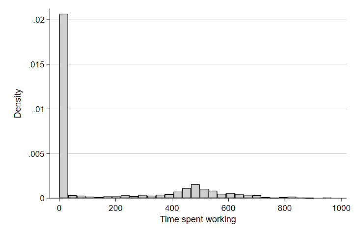
There are two things that jump out here. First, there is a huge pile-up at zero - which means there are a lot of observations that did not work at all on the sampled day they completed their time diary. This is common in time diary data for activities that aren’t guaranteed to occur daily (like sleeping, for instance). There are lots of reasons someone might not work on a given day - holidays, weekends and other days off, or being out of the workforce entirely.
The second thing that jumps out is there seems to be a smaller pile-up at around 500 minutes or around 8 hours. That seems sensible given that a common workday in the U.S. is an eight hour shift. Let’s restrict our graph to only include people of prime working age (between 18 and 60 years old).
hist worktime if teage < 60 & teage > 18 & wkend == 0
graph export "output\hist2.png", replace
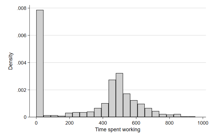
Now that we’ve focused in on people likely to work because they are not retired or too young to work, we have a clearer picture of both the proportion of people who don’t work on a typical day and the distribution of time spent working among those who do.
Let’s take a look at time spent sleeping, a biological function that, of necessity, most people do every day (unless, of course, they are college students cramming for a test or final paper).
hist sleeptime
graph export "output\hist3.png", replace
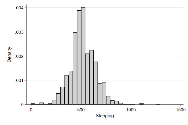
Ah, there’s the approximately normal distribution we might expect from our sample! And again, as we might expect, we see a central tendancy in the distribution to be around 500 or so minutes of sleep in a typical day or about 8 hours.
Okay, so our first reasonable question to ask might be do people with a young child (two years old or less) differ in their time spent at work on a typical day? We might expect to see some dip in dedicating time to work as parents take leave or quit altogether to take care of their young child. Let’s make a bar graph that calculates the average time spent at work separately by having young children and not having young children at home.
graph bar (mean) worktime, over(yngchild) ytitle("Time working")
graph export "output\bar2.png", replace
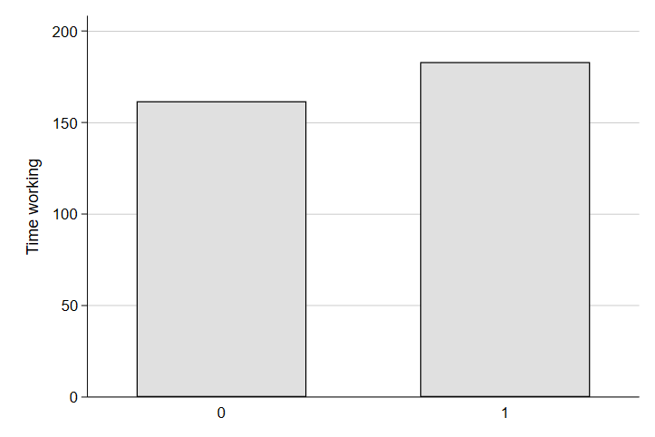
Huh. That’s a little surprising. It seems folks with young children spend more time at work on a typical day than people without young children. Perhaps they extend their working day to add additional income to help cover the costs of the new child. Of course, the burden of parenthood is often inequitable. Indeed, even in Denmark where there are substantial parental leave supports for both fathers and mothers, it is mothers who often take a step back from there careers for meeting parenting needs and this differential burden of parenthood explains a sizeable share of the gender-based wage gap. Moreover, employers often discriminate more against mothers than fathers in reviewing candidates for jobs - further contributing to the gender-based inequity in the professional cost of having a child. Do we see evidence of this in our data? Let’s look at the same difference in work time between people with and without a young child, but this time we will look at the difference separately by gender.
graph bar (mean) worktime, over(yngchild) ytitle("Time working") by(tesex)
graph export "output\bar3.png", replace
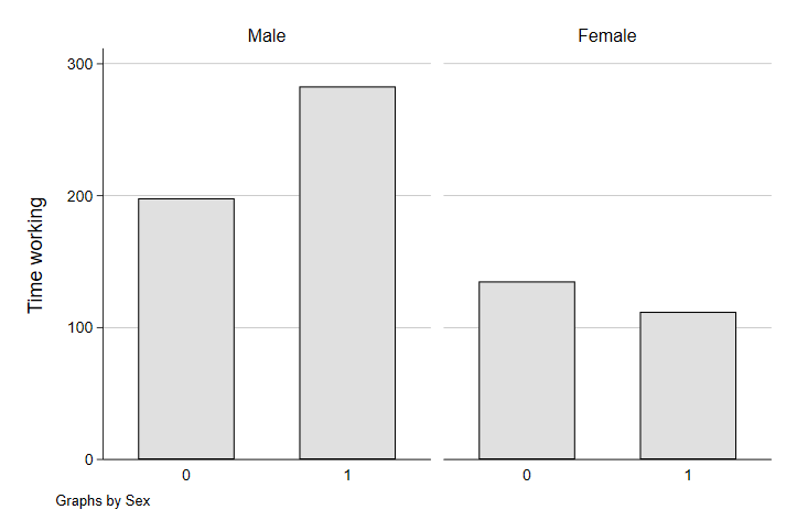
Ah. Now are previous graph makes a little more sense. The combined average of fathers and mothers hides a gender-based difference in the impact of parenthood on time spent working. While fathers up their time at work substantially, mothers seem to take a slight step back in their average time spent working - consistent with the gender-based gap in the effect of parenthood on careers documented in other studies. Fathers taking on more work might be to cover the added costs of the child, to substitute more of their income to compensate for the lost income from mothers reducing their workload for child-rearing, or both. In the aggregate, however, the combination of the two yields workplaces and professions that exhibit a pretty substantial gender-based inequity - something policy-makers may be interested in to try to resolve.
Okay, so what about caretaking? Do women see a bigger uptick in their time spent taking care of children than men?
graph bar (mean) trtcc, over(yngchild) ytitle("Time providing care") by(tesex)
graph export "output\bar4.png", replace
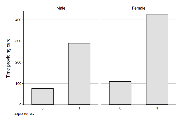
Yep. While both men and women spend more time on caretaking when they have a young child in their household, the childcare burden of a young child seems to be disproportionately born by mothers. Among households without young children (but possibly with older children), the gender gap in childcare time is smaller than when the children are young and childcare is more demanding.
Finally, one concern you might have from this combination of effects is the pressure it puts on couples raising children. If taking a step back from work was not necessarily voluntary, this might be a source of tension. That tension might be exacerbated by inequities in the childcare burden too. One more straing might be a decline in the time couples spend alone with each other when there’s a young child in their household. Let’s take a look at the average time spent alone with a spouse - an indicator of quality time together - separately by whether there is a young child in the household.
graph bar (mean) trtsponly, over(yngchild) ytitle("Time with spouse")
graph export "output\bar5.png", replace
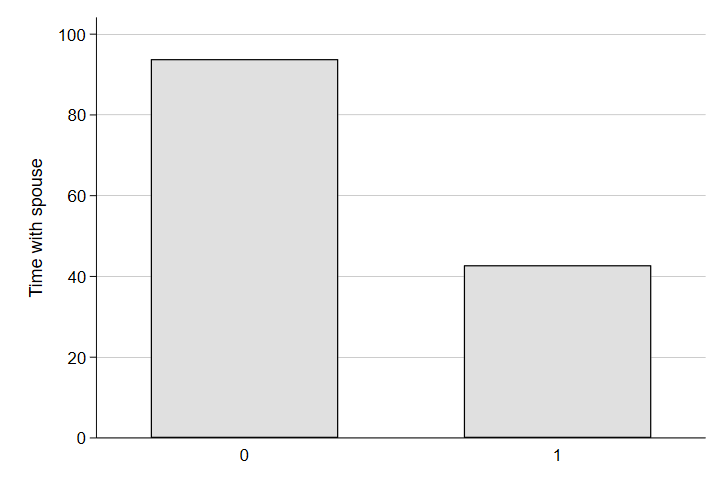
Wow. That’s quite a difference in quality time together! Clearly having a child puts a lot of pressure on a relationship - pressure that can be made worse or ameliorated by various aspects of our policy environment, society, and economy.
Making Tables
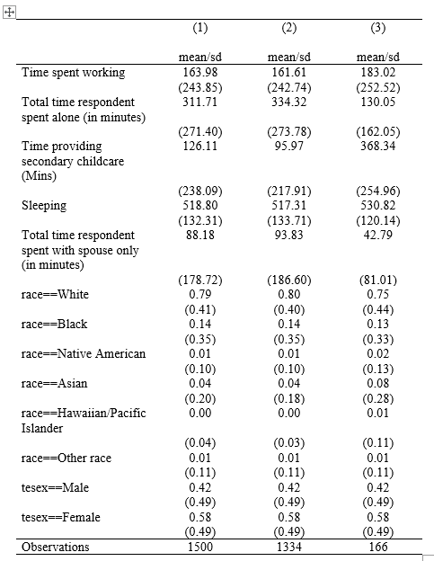
Graphs are great ways to look at the relationship between variables and to summarize individual variables. However, tables are a great way to look at a richer set of information quickly and in one place. Unfortunately, when we run commands in STATA, it’s difficult to share that information outside of our screens. For that, we need to use estout commands that we installed earlier to create nice tables in formats compatable with sharing. For this example, we will look at our same set of time use variables overall and by whether or not there is a young child present in the household. We will also add race and gender to the table to see how representative our sample is demographically overall.
Let’s start by creating indicator variables for each category in race and tesex. We do this because when you take the mean of a variable that only has values of 0 or 1 and multiply it by 100, you have the proportion of your sample in the 1 category. So, for instance, if instead of tesex with values of 1 for men and 2 for women, we have a variable male equal to 0 for women and 1 for mean, that mean of male $\times$ 100 would be the percent of observations that are men. One shortcut to doing this for variables with many categories (e.g., race) is to add a gen(stub) option after a tab command. STATA will then create indicator variables for each category and name them stub# (usually the name of the variable) and the numeric order in which that category appeared in the original variable. Let’s run that real quick.
. tab race, gen(race)

                     Race |      Freq.     Percent        Cum.
--------------------------+-----------------------------------
                    White |      1,189       79.27       79.27
                    Black |        214       14.27       93.53
          Native American |         16        1.07       94.60
                    Asian |         61        4.07       98.67
Hawaiian/Pacific Islander |          3        0.20       98.87
               Other race |         17        1.13      100.00
--------------------------+-----------------------------------
                    Total |      1,500      100.00

. tab tesex, gen(sex)

        Sex |      Freq.     Percent        Cum.
------------+-----------------------------------
       Male |        632       42.13       42.13
     Female |        868       57.87      100.00
------------+-----------------------------------
      Total |      1,500      100.00
You’ll notice after running this, there are six new race variables - race1 through race6 - and two sex variables. These correspond to the categories in race and tesex you see in the tabulation (e.g., race1 is White, race2 is Black, etc.).
Now we have the ingredients we need for our table. I am going to walk through the line by line code of a table, but you will run this as a chunk of code in a .do file.
We will start by running the sum command to summarize all of the variables we want in our table. But first, we will add estpost to the beginning of the code to tell STATA to store the statistics we calculate in its temporary memory. The basic structure of this command will be estpost sum varlist where varlist is a list of all variables we want in our table. Each time we run this, we will be creating new columns in our table and, in general, we will want to use the same list of variables every time and will only be adding or changing if conditions to the end. Let’s begin.
estpost sum worktime trtalone trtcc sleeptime trtsponly race1 race2 race3 race4 race5 race6 sex1 sex2
Here, we calculate the mean, standard deviation, count of observations, and a number of other basic statistics describing each variable we want in our table (time spent working, time alone, time in childcate, sleeping time, time with a spouse, and then our race and gender indicators). Now we are going to add a line that tells labels these estimates so we can call them back later.
est sto all
In that command, est sto is the command and all is a label that we choose - something that reflects the sample from which the estimates are derived. I used all here because the estimates are for the full sample or all observations. The first column of our table will be the summary statistics of all the variables in varlist for the full sample. Each row will be a different variable.
Next, we are going to want to run the estimates for only the folks in our sample who do not have a young child. This will be the second column of our table and remember we want to keep the varlist the same.
estpost sum worktime trtalone trtcc sleeptime trtsponly race1 race2 race3 race4 race5 race6 sex1 sex2 if yngchild == 0
Notice that the command is the same, but I have added an if condition to tell STATA that this time, it should only include observations where there is no young child in the household when calculating the summary statistics. In essence, this changes the denominator of our mean calculations. Let’s label these estimates too.
est sto nochild
Next, we’ll do the same thing again for our third column, but we will replace the 0 with a 1 in the if condition - that way STATA only includes observations with a young child in the household.
estpost sum worktime trtalone trtcc sleeptime trtsponly race1 race2 race3 race4 race5 race6 sex1 sex2 if yngchild == 1
est sto child
Finally, I need to take the labeled estimates (all, nochild, child) and output the statistics I want into a clean, three column table in a word format (in this case .rtf or rich-text format, which word processors can read). The first part of the command is somewhat intuitive: esttab all nochild child using "output\table1.rtf". In that command, I have told STATA to use the esttab command to create a table named table 1, saved to my output folder, in a rtf format, with the columns being the statistics labeled all, nochild, and child in that order. The tricky part is the options. Here, we only really want a measure of central tendancy (the mean) and a measure of spread (the standard deviation) in our tabel. We will use the cell option to tell STATA what statistics should be in the cells of our table and in what order they should appear (mean first, standard deviation second). We will also tell STATA to round to 2 decimal points using the fmt() option and to differentiate standard deviations with parentheses using the par option. Finally, we’ll tell STATA to use labels and add a replace line in case we’ve made this table before. The full line will look like this:
esttab all nochild child using "output\table1.rtf", cell(mean(fmt(2)) sd(fmt(2) par)) label replace
Now, the main to remember is that you can keep code and use it as a sort of template for tables going forward. You don’t have to create everything from scratch - start with code from an old table and change the variable list in and table name and you can re-use the code over and over. It’s one of the big benefits of using code in the first place! The full code that you will run to create the table should look like this:
estpost sum worktime trtalone trtcc sleeptime trtsponly race1 race2 race3 race4 race5 race6 sex1 sex2
est sto all
estpost sum worktime trtalone trtcc sleeptime trtsponly race1 race2 race3 race4 race5 race6 sex1 sex2 if yngchild == 0
est sto nochild
estpost sum worktime trtalone trtcc sleeptime trtsponly race1 race2 race3 race4 race5 race6 sex1 sex2 if yngchild == 1
est sto child
esttab all nochild child using "output\table1.rtf", cell(mean(fmt(2)) sd(fmt(2) par)) label replace
And it should create a nice, clean table that looks like this:
Regressions in STATA
Often, we want to be able to look more precisely that the relationship of interest to us than simply eyeballing bars in a graph or looking at summary statistics across groups. Moreover, we want to know whether the difference we are seeing is random noise or likely a “real” difference.
Let’s start with a simple regression of having a young child on time spent working. The regression version of this relationship would be:
$T_i = \beta_0 + \beta_1 Child_i + \varepsilon_i$
where $T$ is work time and $Child_i$ is an indicator for whether person $i$ has a young child in their household. Since $Child_i$ is an indicator variable, $\beta_1$, the parameter we care about, captures the difference in mean time spent working between people with and without a young child in their household. To run this model in STATA, we would use the reg command. The reg command will always have the structure of reg y x where y is a single outcome variable and x is one or more independent variables. Because yngchild is an indicator variable, we will add an i. in front of it to tell STATA to run it as a categorical variable. Let’s take a look.
reg worktime i.yngchild

      Source |       SS           df       MS      Number of obs   =     1,500
-------------+----------------------------------   F(1, 1498)      =      1.14
       Model |   67696.195         1   67696.195   Prob > F        =    0.2861
    Residual |  89067843.2     1,498  59457.8393   R-squared       =    0.0008
-------------+----------------------------------   Adj R-squared   =    0.0001
       Total |  89135539.4     1,499  59463.3352   Root MSE        =    243.84

------------------------------------------------------------------------------
    worktime | Coefficient  Std. err.      t    P>|t|     [95% conf. interval]
-------------+----------------------------------------------------------------
  1.yngchild |    21.4139   20.06865     1.07   0.286    -17.95174    60.77955
       _cons |   161.6102   6.676159    24.21   0.000     148.5146    174.7058
------------------------------------------------------------------------------
In the output, we can see several things. First, there is indeed a positive difference in time spent working between people with and people without a young child. The coefficient on young child tells us that, relative to people without a young child, people with a young child present spend 21 minutes more working on average.
BUT! Can we be sure that this difference is statistically meaningful? If the true underlying difference in the population was zero, would we be likely to see a difference like this in samples of 1,500 people just by random chance? If we look at the t-statistic and the p-value, we can see that we can’t really be confident that this is not due to random change. The p-value is 0.28, which tells us that 28% of samples would have a difference of 21 minutes if they were drawn from a population where the true underlying difference was 0. That’s not a small enough share for us to confidently reject the null hypothesis of no difference in work time.
Let’s add a control variable to our model - gender. We know gender has an impact on labor market participation and time spent working on a typical day. Gender might also differentially relate to the likelihood of having a young child in the household. If it does both, at least some of the worktime that our model attributes to having a yound child may instead be related to gender.
reg worktime i.yngchild i.sex2

      Source |       SS           df       MS      Number of obs   =     1,500
-------------+----------------------------------   F(2, 1497)      =     18.23
       Model |  2119792.68         2  1059896.34   Prob > F        =    0.0000
    Residual |  87015746.7     1,497  58126.7513   R-squared       =    0.0238
-------------+----------------------------------   Adj R-squared   =    0.0225
       Total |  89135539.4     1,499  59463.3352   Root MSE        =    241.09

------------------------------------------------------------------------------
    worktime | Coefficient  Std. err.      t    P>|t|     [95% conf. interval]
-------------+----------------------------------------------------------------
  1.yngchild |   21.89154   19.84291     1.10   0.270    -17.03131    60.81439
      1.sex2 |  -74.90825   12.60721    -5.94   0.000    -99.63792   -50.17859
       _cons |   204.9042   9.831885    20.84   0.000     185.6185      224.19
------------------------------------------------------------------------------
As we can see, the coefficient on young child did go up a little bit - consistent with the possibility that omitting gender from the models biased our estimates downword a bit. We can also that women work a lot less on a typical day then men. None of this, of course, gives us any insight on the relative effect of a young child on the work time of men versus women. For that, we need to estimate an interaction model.
Interaction Models
Interaction models are a little tricky to interpret at first and people get tripped up on them all the time. However, it’s important to understand interaction terms because they lie at the heart of causal inference. Indeed, a difference-in-difference estimator is a particular application of an interaction regression and interactions estimate a difference in the differences of two groups. In our context, exploring the difference between men and women in the time spent working on a typical day when there’s a young child present, we would be esitmating a regression that looks like this:
$T_i = \alpha + \beta Child_i + \gamma Female_i + \delta Child_i \times Female_i + \varepsilon_i$
Here, think of $Child_i$ and $Female_i$ as switches that turn on when a respondent has a young child present or when a respondent is a woman (or both). The table below gives you a breakdown of how to interpret the coefficients in terms of $E(Y)$ or the average worktime we would expect on a typical day for the various combinations of these two variables.
| Men | Women | |
| No young child | $\alpha$ | $\alpha + \gamma$ |
| Young child | $\alpha + \beta$ | $\alpha + \beta + \gamma + \delta$ |
Notice that the margin for women with a young child relative to women without a child and men with a young child is $\delta$. Put another way, the only parameter that is unique to women with a young child and doesn’t appear for any other group is $\delta$ or the parameter that represents the interaction term in our regression model of worktime as a function of both gender and parenthood. This captures the difference between men and women in average time spent working on a typical day that is unrelated to gender and instead attributable to the gender-based difference in the impact of a young child. If $\delta$ were 0 on average, it would suggest that young children have a similar impact on work time among men and women and the primary difference in work time would be gender-based differences in labor markets (i.e., just $\gamma$, which is relevant to women regardless of having a young child). If, however, $\delta$ is negative, it would suggest that even after accounting for gender differences in the labor market, women have a stronger negative impact on their typical work day from the presence of young children in their household relative to men. More specifically, $\delta$ is capturing the difference in the difference between men and women with and without children or:
$\delta = (Y_{female,child} - Y_{female,nochild}) - (Y_{male,child} - Y_{male,nochild})$
Okay, enough abstract math, let’s see some estimates. We’ll start by looking at our regression estimates and then we will confirm our intuition by looking at average work time among men and women with and without young children.
reg worktime i.yngchild i.sex2 i.yngchild##i.sex2

      Source |       SS           df       MS      Number of obs   =     1,500
-------------+----------------------------------   F(3, 1496)      =     14.61
       Model |  2537728.67         3  845909.556   Prob > F        =    0.0000
    Residual |  86597810.7     1,496  57886.2371   R-squared       =    0.0285
-------------+----------------------------------   Adj R-squared   =    0.0265
       Total |  89135539.4     1,499  59463.3352   Root MSE        =     240.6

-------------------------------------------------------------------------------
     worktime | Coefficient  Std. err.      t    P>|t|     [95% conf. interval]
--------------+----------------------------------------------------------------
   1.yngchild |    84.8864   30.68792     2.77   0.006     24.69048    145.0823
       1.sex2 |  -63.00848    13.3378    -4.72   0.000    -89.17126   -36.84571
              |
yngchild#sex2 |
         1 1  |  -107.9355   40.16956    -2.69   0.007    -186.7301   -29.14085
              |
        _cons |   198.0266    10.1399    19.53   0.000     178.1367    217.9166
-------------------------------------------------------------------------------
In our code, i.yngchild estimates $\beta$, i.sex2 estimates $\gamma$, and i.yngchild##i.sex2 estimates $\delta$. In the output, our constant (_cons) is an estimate of $\alpha$. Here, our results tell us young children have a stronger negative effect on women’s work time than men’s work time. Specifically, relative to a young child’s effect on men’s work time, a woman with a young child can expect to work 107 fewer minutes (or about an hour and 47 minutes less) on a typical day. That’s a sizable impact on women’s careers! Let’s decompose this a bit into the constituent parts to see the intuition of our interpretation. First, let’s look at the average work time of men with and without a child.
Here’s without:
mean worktime if yngchild == 0 & sex2 == 0

Mean estimation                            Number of obs = 563

--------------------------------------------------------------
             |       Mean   Std. err.     [95% conf. interval]
-------------+------------------------------------------------
    worktime |   198.0266   10.98849      176.4431    219.6102
--------------------------------------------------------------
Notice that this is exactly the same as our _cons estimate of $\alpha$ in our regression! Men without a young child work 198 minutes on a typical day.
Here’s men with a young child:
mean worktime if yngchild == 1 & sex2 == 0

Mean estimation                             Number of obs = 69

--------------------------------------------------------------
             |       Mean   Std. err.     [95% conf. interval]
-------------+------------------------------------------------
    worktime |    282.913   34.10085      214.8659    350.9602
--------------------------------------------------------------
Men with a young child work more on average than men without a young child, perhaps to cover the additional costs of parenthood and perhaps to offset the loss of income to childcare. Notice that in our table, men with a young child should work $\alpha + \beta$ minutes. If we add our estimate of $\alpha$ (198.0266) and our estimate of $\beta$ (84.8864), we would have 282.913! This helps underscore that $\beta$ is capturing the difference in average work time between men with and men without young children ($Y_{male,child} - Y_{male,nochild}$).
Now let’s do the same for women. Let’s start with women without children, which should be equal to $\alpha + \gamma$.
mean worktime if yngchild == 0 & sex2 == 1

Mean estimation                            Number of obs = 771

--------------------------------------------------------------
             |       Mean   Std. err.     [95% conf. interval]
-------------+------------------------------------------------
    worktime |   135.0182   8.110284      119.0973     150.939
--------------------------------------------------------------
Women without a young child work less than men without a young child, on average. Once again, we can see that the coefficient on women captures the difference between men without a child (198.0266 or the constant) and women without a young child (135.0182). Holding constant not having a young child, subtracting the average of men from the average of women leaves us with -63.00848 or the estimate of $\gamma$ in our regression!
Alright, now the last piece - women with a young child:
mean worktime if yngchild == 1 & sex2 == 1

Mean estimation                             Number of obs = 97

--------------------------------------------------------------
             |       Mean   Std. err.     [95% conf. interval]
-------------+------------------------------------------------
    worktime |   111.9691   20.43064      71.41457    152.5236
--------------------------------------------------------------
Now we have all our ingredients for calculating the differential effect of a young child on women’s work life relative to men. Intuitively, we would want to know if the difference in work time with and without a young child among men is larger or smaller than the difference in work time with and without a young child among women. For women, this difference is 111.9691 - 135.0182 or -23.0491. For men, the same difference (with child - no child) is 282.913 - 198.0266 or 84.8864. Already, we can kind of see the difference in the effects - among women, the difference is negative and among men the difference is positive. But let’s put a number on this differential effect. We do this by taking the difference among women minus the difference among men. This is -23.0491 - 84.8864 which comes to… ![]()
![]()
![]() …107.9355, exactly our estimate of $\delta$!
…107.9355, exactly our estimate of $\delta$!
This could mean many things of course, but it is consistent with what we observe in the labor market - women receive a pretty large professional penalty from parenthood and the wage gap increases, in part, due to women reducing their work time in response to a young child while men increase their work time. These differences are likely related to gendered cultural expectations about parenting and policy choices that don’t provide the childcare infrastructure to mitigate these effects.
Let’s add some controls to our model and see how income or household size might factor in to this equation.
reg worktime i.yngchild i.sex2 i.yngchild##i.sex2 hhsize highincome

      Source |       SS           df       MS      Number of obs   =     1,500
-------------+----------------------------------   F(5, 1494)      =      9.26
       Model |  2680658.66         5  536131.731   Prob > F        =    0.0000
    Residual |  86454880.7     1,494  57868.0594   R-squared       =    0.0301
-------------+----------------------------------   Adj R-squared   =    0.0268
       Total |  89135539.4     1,499  59463.3352   Root MSE        =    240.56

-------------------------------------------------------------------------------
     worktime | Coefficient  Std. err.      t    P>|t|     [95% conf. interval]
--------------+----------------------------------------------------------------
   1.yngchild |   71.87172   31.95901     2.25   0.025     9.182431     134.561
       1.sex2 |  -62.88245   13.33625    -4.72   0.000    -89.04222   -36.72269
              |
yngchild#sex2 |
         1 1  |  -106.4149   40.18516    -2.65   0.008    -185.2403   -27.58962
              |
       hhsize |    7.03456   4.570611     1.54   0.124    -1.930937    16.00006
   highincome |   3.740078   28.76724     0.13   0.897    -52.68838    60.16854
        _cons |   179.9465   15.35094    11.72   0.000     149.8348    210.0582
-------------------------------------------------------------------------------
The answer is they don’t change our estimated differential effect by much.
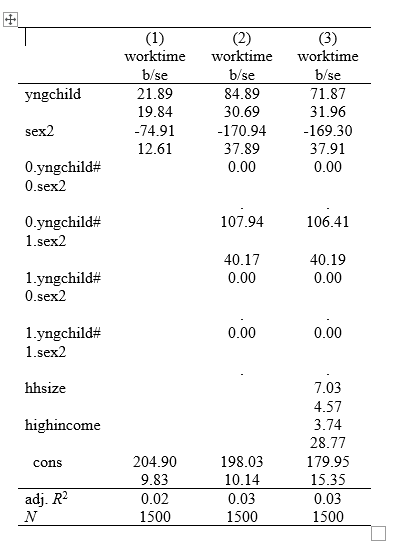
Finally, let’s re-estimate things to create a nice, clean table for use in a report. We will start by showing the impact of young children and gender on work time, then add the interaction between the two, and finally we will add some controls. Our full code will look like this:
reg worktime yngchild sex2
est sto m1
reg worktime yngchild sex2 yngchild#sex2
est sto m2
reg worktime yngchild sex2 yngchild#sex2 hhsize highincome
est sto m3
esttab m1 m2 m3 using "output\table2.rtf", cell(b(fmt(2)) se(par)) ar2(2) obslast compress replace
And our final table should look like this:
We can delete the 0. rows that are empty (nuissance output from Stata) and rename our rows to make them clearer and viola:
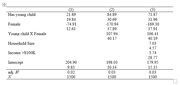
We have a nice table for our report!